The recommended way to run C-PAC is through the use of a container such as Docker or Singularity. Using these containers can be facilitated by cpac (Python package). C-PAC is also available as a .
Containers are completely pre-built environments that help ensure reproducibility (same exact library versions, behavior, etc.).
Docker is the more common option, but may require administrative rights on your system. This is a good option for personal machines.
Singularity is the preferred option for shared resources like servers and clusters with many users. Either you or a system administrator can pull a C-PAC Singularity container for global use across your lab or organization.
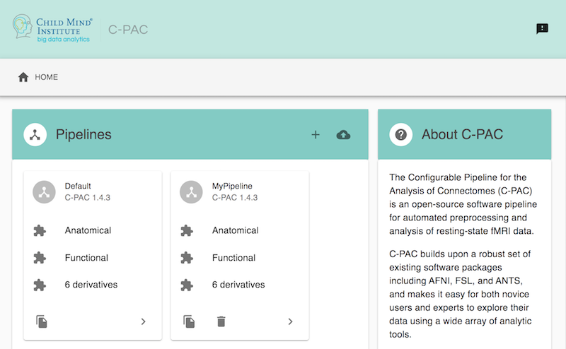
C-PAC comes pre-packaged with a default pipeline, as well as a growing library of pre-configured pipelines. You can use these to get started right away.
However, you can edit any of these pipelines, or build your own from scratch, using our pipeline builder.
C-PAC can also pull input data from the cloud (AWS S3 buckets), so you can pull public data from any of the open-data releases immediately.
More information regarding all of these points are available below, and throughout the rest of the User Guide.
cpac is available so that you can easily run analyses without needing interact with the container platform that allows you to run C-PAC without installing all of the underlying software.
cpac requires Python 3.6 or greater. To get cpac, simply
When downloading/upgrading, the --platform, --image, and --tag let you specify platform (Docker or Singularity), image (Docker image name or URL to image in repository), and tag (version tag, currently only for Docker repositories), respectively.
For example, a development Docker image can be downloaded with
cpac --platform docker --tag nightly pull
Or a Singularity image built from that Docker image can be downloaded with
To run C-PAC in participant mode for one participant, using a BIDS dataset stored on your machine or server and using the container image’s default pipeline configuration:
cpac run /Users/You/local_bids_data /Users/You/some_folder_for_outputs participant
By default, cpac (the wrapper) will try Docker first and fall back to Singularity if Docker fails. If both fail, an exception is raised.
You can specify a platform with the --platformdocker or --platformsingularity. If you specify a platform without specifying an image, these are the defaults, using the first successfully found image:
$ cpac --help
usage: cpac [-h] [--version] [-o OPT] [-B CUSTOM_BINDING] [--platform {docker,singularity}] [--image IMAGE] [--tag TAG] [--working_dir PATH] [-v] [-vv] {run,group,utils,pull,upgrade,crash} ...cpac: a Python package that simplifies using C-PAC <http://fcp-indi.github.io> containerized images.This commandline interface package is designed to minimize repetition.As such, nearly all arguments are optional.When launching a container, this package will try to bind any paths mentioned in • the command • the data configurationAn example minimal run command: cpac run /path/to/data /path/for/outputsAn example run command with optional arguments: cpac -B /path/to/data/configs:/configs \ --image fcpindi/c-pac --tag latest \ run /path/to/data /path/for/outputs \ --data_config_file /configs/data_config.yml \ --save_working_dirEach command can take "--help" to provide additonal usage information, e.g., cpac run --helppositional arguments: {run,group,utils,pull,upgrade,crash}optional arguments: -h, --help show this help message and exit --version show program's version number and exit -o OPT, --container_option OPT parameters and flags to pass through to Docker or Singularity This flag can take multiple arguments so cannot be the final argument before the command argument (i.e., run or any other command that does not start with - or --) -B CUSTOM_BINDING, --custom_binding CUSTOM_BINDING directories to bind with a different path in the container than the real path of the directory. One or more pairs in the format: real_path:container_path (eg, /home/C-PAC/run5/outputs:/outputs). Use absolute paths for both paths. This flag can take multiple arguments so cannot be the final argument before the command argument (i.e., run or any other command that does not start with - or --) --platform {docker,singularity} If neither platform nor image is specified, cpac will try Docker first, then try Singularity if Docker fails. --image IMAGE path to Singularity image file OR name of Docker image (eg, "fcpindi/c-pac"). Will attempt to pull from Singularity Hub or Docker Hub if not provided. If image is specified but platform is not, platform is assumed to be Singularity if image is a path or Docker if image is an image name. --tag TAG tag of the Docker image to use (eg, "latest" or "nightly"). --working_dir PATH working directory -v, --verbose set loglevel to INFO -vv, --very-verbose set loglevel to DEBUG
Look in the present working directory for any Singularity images. If more than one is found, use the most recently modified.
Pull FCP-INDI/C-PAC from Singularity Hub.
Pull fcpindi/c-pac:latest from Docker Hub and convert to a Singularity image.
You can also specify a container image with an --image argument, passing an image name (e.g., fcpindi/c-pac) for a Docker image or a filepath (e.g. ~/singularity_images/C-PAC.sif) for a Singularity image. You can also specify a --tag (e.g., latest or nightly).
You can also provide a link to an AWS S3 bucket containing a BIDS directory as the data source:
cpac run s3://fcp-indi/data/Projects/ADHD200/RawDataBIDS /Users/You/some_folder_for_outputs participant
In addition to the default pipeline, C-PAC comes packaged with a growing library of pre-configured pipelines that are ready to use. To run C-PAC with one of the pre-packaged pre-configured pipelines, simply invoke the --preconfig flag, shown below. See the full selection of pre-configured pipelines here.
cpac run /Users/You/local_bids_data /Users/You/some_folder_for_outputs --preconfig anat-only
To run C-PAC with a pipeline configuration file other than one of the pre-configured pipelines, assuming the configuration file is in the /Users/You/Documents directory:
cpac run /Users/You/local_bids_data /Users/You/some_folder_for_outputs participant --pipeline_file /Users/You/Documents/pipeline_config.yml
Finally, to run C-PAC with a specific data configuration file (instead of providing a BIDS data directory):
cpac run /Users/You/any_directory /Users/You/some_folder_for_outputs participant --data_config_file /Users/You/Documents/data_config.yml
Note: we are still providing the postionally-required bids_dir input parameter. However C-PAC will not look for data in this directory when you provide a data configuration YAML with the --data_config_file flag. Providing . or $PWD will simply pass the present working directory. In addition, if the dataset in your data configuration file is not in BIDS format, just make sure to add the --skip_bids_validator flag at the end of your command to bypass the BIDS validation process.
The full list of parameters and options that can be passed to C-PAC are shown below:
$ cpac run --help
Loading 🐳 DockerLoading 🐳 fcpindi/c-pac:latest with these directory bindings: local Docker mode ---------------------------- -------------------- ------ /home/circleci/build /home/circleci/build rw /home/circleci/build /tmp rw /home/circleci/build/log /logs rw /home/circleci/build/outputs /output rwLogging messages will refer to the Docker paths.usage: run.py [-h] [--pipeline_file PIPELINE_FILE] [--group_file GROUP_FILE] [--data_config_file DATA_CONFIG_FILE] [--preconfig PRECONFIG] [--aws_input_creds AWS_INPUT_CREDS] [--aws_output_creds AWS_OUTPUT_CREDS] [--n_cpus N_CPUS] [--mem_mb MEM_MB] [--mem_gb MEM_GB] [--num_ants_threads NUM_ANTS_THREADS] [--random_seed RANDOM_SEED] [--save_working_dir [SAVE_WORKING_DIR]] [--disable_file_logging] [--participant_label PARTICIPANT_LABEL [PARTICIPANT_LABEL ...]] [--participant_ndx PARTICIPANT_NDX] [--T1w_label T1W_LABEL] [--bold_label BOLD_LABEL [BOLD_LABEL ...]] [-v] [--bids_validator_config BIDS_VALIDATOR_CONFIG] [--skip_bids_validator] [--anat_only] [--tracking_opt-out] [--monitoring] bids_dir output_dir {participant,group,test_config,cli}C-PAC Pipeline Runnerpositional arguments: bids_dir The directory with the input dataset formatted according to the BIDS standard. Use the format s3://bucket/path/to/bidsdir to read data directly from an S3 bucket. This may require AWS S3 credentials specified via the --aws_input_creds option. output_dir The directory where the output files should be stored. If you are running group level analysis this folder should be prepopulated with the results of the participant level analysis. Use the format s3://bucket/path/to/bidsdir to write data directly to an S3 bucket. This may require AWS S3 credentials specified via the --aws_output_creds option. {participant,group,test_config,cli} Level of the analysis that will be performed. Multiple participant level analyses can be run independently (in parallel) using the same output_dir. test_config will run through the entire configuration process but will not execute the pipeline.optional arguments: -h, --help show this help message and exit --pipeline_file PIPELINE_FILE Path for the pipeline configuration file to use. Use the format s3://bucket/path/to/pipeline_file to read data directly from an S3 bucket. This may require AWS S3 credentials specified via the --aws_input_creds option. --group_file GROUP_FILE Path for the group analysis configuration file to use. Use the format s3://bucket/path/to/pipeline_file to read data directly from an S3 bucket. This may require AWS S3 credentials specified via the --aws_input_creds option. The output directory needs to refer to the output of a preprocessing individual pipeline. --data_config_file DATA_CONFIG_FILE Yaml file containing the location of the data that is to be processed. This file is not necessary if the data in bids_dir is organized according to the BIDS format. This enables support for legacy data organization and cloud based storage. A bids_dir must still be specified when using this option, but its value will be ignored. Use the format s3://bucket/path/to/data_config_file to read data directly from an S3 bucket. This may require AWS S3 credentials specified via the --aws_input_creds option. --preconfig PRECONFIG Name of the pre-configured pipeline to run. --aws_input_creds AWS_INPUT_CREDS Credentials for reading from S3. If not provided and s3 paths are specified in the data config we will try to access the bucket anonymously use the string "env" to indicate that input credentials should read from the environment. (E.g. when using AWS iam roles). --aws_output_creds AWS_OUTPUT_CREDS Credentials for writing to S3. If not provided and s3 paths are specified in the output directory we will try to access the bucket anonymously use the string "env" to indicate that output credentials should read from the environment. (E.g. when using AWS iam roles). --n_cpus N_CPUS Number of execution resources per participant available for the pipeline. This flag takes precidence over max_cores_per_participant in the pipeline configuration file. --mem_mb MEM_MB Amount of RAM available per participant in megabytes. Included for compatibility with BIDS-Apps standard, but mem_gb is preferred. This flag takes precedence over maximum_memory_per_participant in the pipeline configuration file. --mem_gb MEM_GB Amount of RAM available per participant in gigabytes. If this is specified along with mem_mb, this flag will take precedence. This flag also takes precedence over maximum_memory_per_participant in the pipeline configuration file. --num_ants_threads NUM_ANTS_THREADS The number of cores to allocate to ANTS-based anatomical registration per participant. Multiple cores can greatly speed up this preprocessing step. This number cannot be greater than the number of cores per participant. --random_seed RANDOM_SEED Random seed used to fix the state of execution. If unset, each process uses its own default. If set, a `random.log` file will be generated logging the random state used by each process. If set to a positive integer (up to 2147483647), that integer will be used to seed each process. If set to 'random', a random seed will be generated and recorded for each process. --save_working_dir [SAVE_WORKING_DIR] Save the contents of the working directory. --disable_file_logging Disable file logging, this is useful for clusters that have disabled file locking. --participant_label PARTICIPANT_LABEL [PARTICIPANT_LABEL ...] The label of the participant that should be analyzed. The label corresponds to sub-<participant_label> from the BIDS spec (so it does not include "sub-"). If this parameter is not provided all participants should be analyzed. Multiple participants can be specified with a space separated list. --participant_ndx PARTICIPANT_NDX The index of the participant that should be analyzed. This corresponds to the index of the participant in the data config file. This was added to make it easier to accommodate SGE array jobs. Only a single participant will be analyzed. Can be used with participant label, in which case it is the index into the list that follows the participant_label flag. Use the value "-1" to indicate that the participant index should be read from the AWS_BATCH_JOB_ARRAY_INDEX environment variable. --T1w_label T1W_LABEL C-PAC only runs one T1w per participant-session at a time, at this time. Use this flag to specify any BIDS entity (e.g., "acq-VNavNorm") or sequence of BIDS entities (e.g., "acq-VNavNorm_run-1") to specify which of multiple T1w files to use. Specify "--T1w_label T1w" to choose the T1w file with the fewest BIDS entities (i.e., the final option of [*_acq- VNavNorm_T1w.nii.gz, *_acq-HCP_T1w.nii.gz, *_T1w.nii.gz"]). C-PAC will choose the first T1w it finds if the user does not provide this flag, or if multiple T1w files match the --T1w_label provided. If multiple T2w files are present and a comparable filter is possible, T2w files will be filtered as well. If no T2w files match this --T1w_label, T2w files will be processed as if no --T1w_label were provided. --bold_label BOLD_LABEL [BOLD_LABEL ...] To include a specified subset of available BOLD files, use this flag to specify any BIDS entity (e.g., "task- rest") or sequence of BIDS entities (e.g. "task- rest_run-1"). To specify the bold file with the fewest BIDS entities in the file name, specify "--bold_label bold". Multiple `--bold_label`s can be specified with a space-separated list. If multiple `--bold_label`s are provided (e.g., "--bold_label task-rest_run-1 task-rest_run-2", each scan that includes all BIDS entities specified in any of the provided `--bold_label`s will be analyzed. If this parameter is not provided all BOLD scans should be analyzed. -v, --version show program's version number and exit --bids_validator_config BIDS_VALIDATOR_CONFIG JSON file specifying configuration of bids-validator: See https://github.com/bids-standard/bids-validator for more info. --skip_bids_validator Skips bids validation. --anat_only run only the anatomical preprocessing --tracking_opt-out Disable usage tracking. Only the number of participants on the analysis is tracked. --monitoring Enable monitoring server on port 8080. You need to bind the port using the Docker flag "-p".
$ cpac utils --help
Loading 🐳 DockerLoading 🐳 fcpindi/c-pac:latest with these directory bindings: local Docker mode ---------------------------- -------------------- ------ /home/circleci/build /home/circleci/build rw /home/circleci/build /tmp rw /home/circleci/build/outputs /output rw /home/circleci/build/log /logs rwLogging messages will refer to the Docker paths.Usage: run.py utils [OPTIONS] COMMAND [ARGS]...Options: --help Show this message and exit.Commands: crash data_config group_config pipe_config repickle test tools workflows
Note that any of the optional arguments above will over-ride any pipeline settings in the default pipeline or in the pipeline configuration file you provide via the --pipeline_file parameter.
Further usage notes:
You can run only anatomical preprocessing easily, without modifying your data or pipeline configuration files, by providing the --anat_only flag.
As stated, the default behavior is to read data that is organized in the BIDS format. This includes data that is in Amazon AWS S3 by using the format s3://<bucket_name>/<bids_dir> for the bids_dir command line argument. Outputs can be written to S3 using the same format for the output_dir. Credentials for accessing these buckets can be specified on the command line (using --aws_input_creds or --aws_output_creds).
When the app is run, a data configuration file is written to the working directory. This directory can be specified with --working_dir or the directory from which you run cpac will be used. This file can be passed into subsequent runs, which avoids the overhead of re-parsing the BIDS input directory on each run (i.e. for cluster or cloud runs). These files can be generated without executing the C-PAC pipeline using the test_run command line argument.
The participant_label and participant_ndx arguments allow the user to specify which of the many datasets should be processed, which is useful when parallelizing the run of multiple participants.
If you want to pass runtime options to your container plaform (Docker or Singularity), you can pass them with -o or --container_options.
Footnotes
For instructions to run C-PAC in Docker or Singularity without installing cpac (Python package), see All Run Options
C-PAC is packaged with a default processing pipeline so that you can get your data preprocessing and analysis started immediately. Just pull the C-PAC Docker container and kick off the container with your data, and you’re on your way.
The default processing pipeline performs fMRI processing using four strategies, with and without global signal regression, with and without bandpass filtering.
Anatomical processing begins with conforming the data to RPI orientation and removing orientation header information that will interfere with further processing. A non-linear transform between skull-on images and a 2mm MNI brain-only template are calculated using ANTs [3]. Images are them skull-stripped using AFNI’s 3dSkullStrip [5] and subsequently segmented into WM, GM, and CSF using FSL’s fast tool [6]. The resulting WM mask was multiplied by a WM prior map that was transformed into individual space using the inverse of the linear transforms previously calculated during the ANTs procedure. A CSF mask was multiplied by a ventricle map derived from the Harvard-Oxford atlas distributed with FSL [4]. Skull-stripped images and grey matter tissue maps are written into MNI space at 2mm resolution.
Functional preprocessing begins with resampling the data to RPI orientation, and slice timing correction. Next, motion correction is performed using a two-stage approach in which the images are first coregistered to the mean fMRI and then a new mean is calculated and used as the target for a second coregistration (AFNI 3dvolreg [2]). A 7 degree of freedom linear transform between the mean fMRI and the structural image is calculated using FSL’s implementation of boundary-based registration [7]. Nuisance variable regression (NVR) is performed on motion corrected data using a 2nd order polynomial, a 24-regressor model of motion [8], 5 nuisance signals, identified via principal components analysis of signals obtained from white matter (CompCor, [9]), and mean CSF signal. WM and CSF signals were extracted using the previously described masks after transforming the fMRI data to match them in 2mm space using the inverse of the linear fMRI-sMRI transform. The NVR procedure is performed twice, with and without the inclusion of the global signal as a nuisance regressor. The residuals of the NVR procedure are processed with and without bandpass filtering (0.001Hz < f < 0.1Hz), written into MNI space at 3mm resolution and subsequently smoothed using a 6mm FWHM kernel.
Several different individual level analysis are performed on the fMRI data including:
Amplitude of low frequency fluctuations (alff) [10]: the variance of each voxel is calculated after bandpass filtering in original space and subsequently written into MNI space at 2mm resolution and spatially smoothed using a 6mm FWHM kernel.
Fractional amplitude of low frequency fluctuations (falff) [11]: Similar to alff except that the variance of the bandpassed signal is divided by the total variance (variance of non-bandpassed signal.
Regional homogeniety (ReHo) [12]: a simultaneous Kendalls correlation is calculated between each voxel’s time course and the time courses of the 27 voxels that are face, edge, and corner touching the voxel. ReHo is calculated in original space and subsequently written into MNI space at 2mm resolution and spatially smoothed using a 6mm FWHM kernel.
Voxel mirrored homotopic connectivity (VMHC) [13]: an non-linear transform is calculated between the skull-on anatomical data and a symmetric brain template in 2mm space. Using this transform, processed fMRI data are written in to symmetric MNI space at 2mm and the correlation between each voxel and its analog in the contralateral hemisphere is calculated. The Fisher transform is applied to the resulting values, which are then spatially smoothed using a 6mm FWHM kernel.
Weighted and binarized degree centrality (DC) [14]: fMRI data is written into MNI space at 2mm resolution and spatially smoothed using a 6mm FWHM kernel. The voxel x voxel similarity matrix is calculated by the correlation between every pair of voxel time courses and then thresholded so that only the top 5% of correlations remain. For each voxel, binarized DC is the number of connections that remain for the voxel after thresholding and weighted DC is the average correlation coefficient across the remaining connections.
Eigenvector centrality (EC) [15]: fMRI data is written into MNI space at 2mm resolution and spatially smoothed using a 6mm FWHM kernel. The voxel x voxel similarity matrix is calculated by the correlation between every pair of voxel time courses and then thresholded so that only the top 5% of correlations remain. Weighted EC is calculated from the eigenvector corresponding to the largest eigenvalue from an eigenvector decomposition of the resulting similarity. Binarized EC, is the first eigenvector of the similarity matrix after setting the non-zero values in the resulting matrix are set to 1.
Local functional connectivity density (lFCD) [16]: fMRI data is written into MNI space at 2mm resolution and spatially smoothed using a 6mm FWHM kernel. For each voxel, lFCD corresponds to the number of contiguous voxels that are correlated with the voxel above 0.6 (r>0.6). This is similar to degree centrality, except only voxels that it only includes the voxels that are directly connected to the seed voxel.
10 intrinsic connectivity networks (ICNs) from dual regression [17]: a template including 10 ICNs from a meta-analysis of resting state and task fMRI data [18] is spatially regressed against the processed fMRI data in MNI space. The resulting time courses are entered into a multiple regression with the voxel data in original space to calculate individual representations of the 10 ICNs. The resulting networks are written into MNI space at 2mm and then spatially smoothed using a 6mm FWHM kernel.
Seed correlation analysis (SCA): preprocessed fMRI data is to match template that includes 160 regions of interest defined from a meta-analysis of different task results [19]. A time series is calculated for each region from the mean of all intra-ROI voxel time series. A separate functional connectivity map is calculated per ROI by correlating its time course with the time courses of every other voxel in the brain. Resulting values are Fisher transformed, written into MNI space at 2mm resolution, and then spatial smoothed using a 6mm FWHM kernel.
Time series extraction: similar the procedure used for time series analysis, the preprocessed functional data is written into MNI space at 2mm and then time series for the various atlases are extracted by averaging within region voxel time courses. This procedure was used to generate summary time series for the automated anatomic labelling atlas [20], Eickhoff-Zilles atlas [21], Harvard-Oxford atlas [22], Talaraich and Tournoux atlas [23], 200 and 400 regions from the spatially constrained clustering voxel timeseries [24], and 160 ROIs from a meta-analysis of task results [19]. Time series for 10 ICNs were extracted using spatial regression.
In addition to the default pipeline, C-PAC comes packaged with a growing library of pre-configured pipelines that are ready to use. They can be invoked when running C-PAC using the --preconfig flag detailed above.
Detailed information about the selection of pre-configured pipelines are available here.
Mappings for all other C-PAC 1.7 keys can be found here.
C-PAC offers a graphical interface you can use to quickly and easily modify the default pipeline or create your own from scratch: https://fcp-indi.github.io/C-PAC_GUI/
Currently the GUI creates a C-PAC v1.6.0 pipeline configuration file. This syntax persisted through v1.7.2 but is deprecated with the release of v1.8.0.
If given a pipeline file in the older syntax, C-PAC v1.8 will attempt to convert the pipeline configuration file to the new syntax, saving the converted file in your output directory.
An update to the GUI to create v1.8.0 syntax configuration files is underway.
The newer (v1.8) syntax will not work with older versions of C-PAC.
We currently have a publication in preparation, in the meantime please cite our poster from INCF:
Craddock C, Sikka S, Cheung B, Khanuja R, Ghosh SS, Yan C, Li Q, Lurie D, Vogelstein J, Burns R, Colcombe S,Mennes M, Kelly C, Di Martino A, Castellanos FX and Milham M (2013). Towards Automated Analysis of Connectomes:The Configurable Pipeline for the Analysis of Connectomes (C-PAC). Front. Neuroinform. Conference Abstract:Neuroinformatics 2013. doi:10.3389/conf.fninf.2013.09.00042@ARTICLE{cpac2013, AUTHOR={Craddock, Cameron and Sikka, Sharad and Cheung, Brian and Khanuja, Ranjeet and Ghosh, Satrajit S and Yan, Chaogan and Li, Qingyang and Lurie, Daniel and Vogelstein, Joshua and Burns, Randal and Colcombe, Stanley and Mennes, Maarten and Kelly, Clare and Di Martino, Adriana and Castellanos, Francisco Xavier and Milham, Michael}, TITLE={Towards Automated Analysis of Connectomes: The {Configurable Pipeline for the Analysis of Connectomes (C-PAC)}}, JOURNAL={Frontiers in Neuroinformatics}, YEAR={2013}, NUMBER={42}, URL={http://www.frontiersin.org/neuroinformatics/10.3389/conf.fninf.2013.09.00042/full}, DOI={10.3389/conf.fninf.2013.09.00042}, ISSN={1662-5196}}
Gorgolewski, K., Burns, C.D., Madison, C., Clark, D., Halchenko, Y.O., Waskom, M.L., Ghosh, S.S.: Nipype: A flexible, lightweight and extensible neuroimaging data processing framework in python. Front. Neuroinform. 5 (2011). doi:10.3389/fninf.2011.00013
Cox, R.W., Jesmanowicz, A.: Real-time 3d image registration for functional mri. Magn Reson Med 42(6), 1014–8 (1999)
Avants, B., Epstein, C., Grossman, M., Gee, J.: Symmetric diffeomorphic image registration with cross-correlation: Evaluating automated labeling of elderly and neurodegenerative brain. Medical Image Analysis 12(1), 26–41 (2008). doi:10.1016/j.media.2007.06.004
Smith, S.M., Jenkinson, M., Woolrich, M.W., Beckmann, C.F., Behrens, T.E.J., Johansen-Berg, H., Bannister, P.R., Luca, M.D., Drobnjak, I., Flitney, D.E., Niazy, R.K., Saunders, J., Vickers, J., Zhang, Y., Stefano, N.D., Brady, J.M., Matthews, P.M.: Advances in functional and structural mr image analysis and implementation as fsl. NeuroImage 23, 208–219 (2004). doi:10.1016/j.neuroimage.2004.07.051
Smith, S.M.: Fast robust automated brain extraction. Human Brain Mapping 17(3), 143–155 (2002). doi:10.1002/hbm.10062
Zhang, Y., Brady, M., Smith, S.: Segmentation of brain mr images through a hidden markov random field model and the expectation-maximization algorithm. IEEE Transactions on Medical Imaging 20(1), 45–57 (2001). doi:10.1109/42.906424
Greve, D.N., Fischl, B.: Accurate and robust brain image alignment using boundary-based registration. NeuroImage 48(1), 63–72 (2009). doi:10.1016/j.neuroimage.2009.06.060
Friston, K.J., Williams, S., Howard, R., Frackowiak, R.S., Turner, R.: Movement-related effects in fmri time-series. Magn Reson Med 35(3), 346–55 (1996)
Behzadi, Y., Restom, K., Liau, J., Liu, T.T.: A component based noise correction method (compcor) for bold and perfusion based fmri. NeuroImage 37(1), 90–101 (2007). doi:10.1016/j.neuroimage.2007.04.042
Zang, Y.-F., He, Y., Zhu, C.-Z., Cao, Q.-J., Sui, M.-Q., Liang, M., Tian, L.-X., et al. (2007). Altered baseline brain activity in children with ADHD revealed by resting-state functional MRI. Brain & development, 29(2), 83–91.
Zou, Q.-H., Zhu, C.-Z., Yang, Y., Zuo, X.-N., Long, X.-Y., Cao, Q.-J., Wang, Y.-F., et al. (2008). An improved approach to detection of amplitude of low-frequency fluctuation (ALFF) for resting-state fMRI: Fractional ALFF. Journal of neuroscience methods, 172(1), 137–141.
Stark, D. E., Margulies, D. S., Shehzad, Z. E., Reiss, P., Kelly, A. M. C., Uddin, L. Q., Gee, D. G., et al. (2008). Regional variation in interhemispheric coordination of intrinsic hemodynamic fluctuations. The Journal of Neuroscience, 28(51), 13754–13764.
Buckner RL, Sepulcre J, Talukdar T, Krienen FM, Liu H, Hedden T, Andrews-Hanna JR, Sperling RA, Johnson KA. 2009. Cortical hubs revealed by intrinsic functional connectivity: mapping, assessment of stability, and relation to Alzheimer’s disease. J Neurosci. 29:1860–1873.
Lohmann G, Margulies DS, Horstmann A, Pleger B, Lepsien J, Goldhahn D, Schloegl H, Stumvoll M, Villringer A, Turner R. 2010. Eigenvector centrality mapping for analyzing connectivity patterns in fMRI data of the human brain. PLoS One. 5:e10232
C.F. Beckmann, C.E. Mackay, N. Filippini, and S.M. Smith. Group comparison of resting-state FMRI data using multi-subject ICA and dual regression. OHBM, 2009.
Smith, S. M., Fox, P. T., Miller, K. L., Glahn, D. C., Fox, P. M., Mackay, C. E., et al. (2009). Correspondence of the brain’s functional architecture during activation and rest. Proceedings of the National Academy of Sciences of the United States of America, 106(31), 13040–13045. doi:10.1073/pnas.0905267106
Dosenbach, N. U. F., Nardos, B., Cohen, A. L., Fair, D. a, Power, J. D., Church, J. a, … Schlaggar, B. L. (2010). Prediction of individual brain maturity using fMRI. Science (New York, N.Y.), 329(5997), 1358–61. http://doi.org/10.1126/science.1194144
Tzourio-Mazoyer, N., Landeau, B., Papathanassiou, D., Crivello, F., Etard, O., Delcroix, N., … Joliot, M. (2002). Automated anatomical labeling of activations in SPM using a macroscopic anatomical parcellation of the MNI MRI single-subject brain. NeuroImage, 15(1), 273–89. http://doi.org/10.1006/nimg.2001.0978
Eickhoff, S. B., Stephan, K. E., Mohlberg, H., Grefkes, C., Fink, G. R., Amunts, K., & Zilles, K. (2005). A new SPM toolbox for combining probabilistic cytoarchitectonic maps and functional imaging data. NeuroImage, 25(4), 1325–35. http://doi.org/10.1016/j.neuroimage.2004.12.034
Lancaster, J. L., Woldorff, M. G., Parsons, L. M., Liotti, M., Freitas, C. S., Rainey, L., … Fox, P. T. (2000). Automated Talairach atlas labels for functional brain mapping. Human Brain Mapping, 10(3), 120–31. Retrieved from http://www.ncbi.nlm.nih.gov/pubmed/10912591
Craddock, R. C., James, G. A., Holtzheimer, P. E., Hu, X. P., & Mayberg, H. S. (2011). A whole brain fMRI atlas generated via spatially constrained spectral clustering. Human Brain Mapping, 0(July 2010). http://doi.org/10.1002/hbm.21333
 .
.