Nuisance Signal Regression
A key step in preparing fMRI data for statistical analysis is the removal of nusiance signals and noise. C-PAC provides a number of options for removing nuisance signals. These methods can be combined as desired by you, and are described below.
Regressors
Mean White Matter / CSF
The mean WM and CSF time series are calculated by averaging signal over all voxels within a WM or CSF mask for each time point. Mean WM and CSF time series are then used as temporal covariates and removed from the raw data through linear regression.
Note: The Lateral Ventricles Mask in standard space is provided for isolating signal changes in the CSF. This mask is based off of the HarvardOxford atlas that is in standard MNI space. If you wish to use your own standard and lateral ventricles mask, and wish to run CSF nuisance regression, you must specify it in your pipeline configuration.
aCompCor
The term “noise region-of-interest” (noise ROI) refers to areas such as white matter (WM) and cerebral spinal fluid (CSF) in which temporal fluctuations are unlikely to be modulated by neural activity, and thus primarily reflect physiological noise (Behzadi et al., 2007). Based on the assumption that signal from a noise ROI can be used to accurately model physiological fluctuations in gray matter regions, a novel component based noise reduction method (CompCor) was proposed to correct for physiological noise by regressing out principal components from noise ROIs (Behzadi et al., 2007). Compared to the average signal from WM and CSF regions (i.e. WM/CSF regression methods), signals captured by principal components derived from these noise ROIs can better account for voxel-specific phase differences in physiological noise due to the potential of principle component analysis to identify temporal pattern of physiological noise (Tomas et al., 2002). Thus, preprocessing with CompCor can significantly reduce physiological noise as well as noise from other sources (Behzadi et al., 2007; Chai et al., 2012).
The first step of CompCor is to determine noise ROIs. This can be done either by using anatomical data to identify voxels that consist primarily of either WM or CSF, or by defining noise ROIs as voxels with high temporal standard deviation. A principal component analysis (PCA) is then applied to characterize the time series data from the noise ROIs. Significant principal components are then introduced as covariates in a general linear model (GLM) as an estimate of the physiological noise signal space (Behzadi et al., 2007).
Also, C-PAC allows users configure nuisance correction to perform cosine/linear filtering on the time series data prior to CompCor calculation.
tCompCor
As showed by Lund and Hanson (2001), voxel time courses with a relatively high temporal standard deviation were dominated by physiological noise. Behzadi et al. (2007) proposed an unsupervised method to assess the temporal standard deviation and then used princial components analysis to reduce the data dimensionality.
Global Signal Regression
Global signal, the average signal across all voxels in the brain, is assumed to reflect a combination of resting-state fluctuations, physiological noise (e.g. respiratory and cardiac noise), and other noise signals with non-neural origin. Global signal regression (GSR) is a preprocessing technique for removing the spontaneous BOLD fluctuations common to the whole brain using a general linear model (GLM). Although GSR can potentially change functional connectivity distributions and result in increased negative correlations (Murphy et al., 2009; Saad et al., 2012; Weissenbacher et al., 2009), this technique has been shown to facilitate the detection of localized neuronal signals and improve the specificity of functional connectivity analysis (Fox et al., 2005; Fox et al., 2009). Thus, GSR remains a common and useful processing technique in some situations.
Global Mean
A global mean (defined as the average signal over all voxels for each time point) is used as a temporal covariate and regressed out using linear regression.
Principle Components Removal
Performs a Principal Components Analysis and regresses out the chosen principal component. The first component is assumed to be the global mean signal.
Polynomial Detrending
Removes linear or quadratic trends in the timeseries. The linear trend is likely due to the scanner heating up as the scan progresses, while the quadratic trend is possibly due to slow movement-related effects.
Motion Correction
Movement during scanning is one of of the largest factors influencing the quality of fMRI data. Movement of the head between the acquisition of each volume can cause brain images to become misaligned. Head motion during scanning can also cause spurious changes in signal intensity. If they are not corrected, these changes can influence the results of activation and connectivity analyses. Recent studies have shown that motion as small as 0.1 mm can systematically bias both within- and between- group effects during the analysis of fMRI data (Power et al., 2011; Satterhwaite et al., 2012; Van Dijk et al., 2012). Even the most cooperative participants often still show displacements of up to a millimeter, and head movements of several millimeters are not uncommon in studies of hyperkinetic subjects such as young children, older adults, or patient populations.
There are four main approaches to motion correction: volume realignment, using a general linear model to regress out motion-related artifacts (i.e. regression of motion parameters, as described as one of the regressors in nuisance regression above), de-spiking of motion confounded time points, and censoring of motion confounded time points (i.e. “scrubbing”).
Volume Realignment
Volume realignment aligns reconstructed volumes by calculating motion parameters based on a solid-body model of the head and brain (Friston 1996). Based on these parameters, each volume is registered to the volume preceding it.
C-PAC runs volume realignment on all functional images during functional preprocessing. You can select from two sets of motion parameters to use during this process:
6-Parameter Model - Three translation and three rotation parameters as described in Friston 1996.
Friston 24-Parameter Model - The 6 motion parameters of the current volume and the preceding volume, plus each of these values squared.
Regression of Motion Parameters
Another approach to motion correction is to regress out the effects of motion when running statistical analysis. This is done by calculating motion parameters and including them in your General Linear Model (Fox et al., 2005; Weissenbacher et al., 2009).
By default, C-PAC will calculate and output the motion parameters used during volume realignment. You can optionally enable the calculation of additional motion parameters, including Framewise Displacement (FD) and DVARS (as described below and in Power et al., 2011).
De-Spiking
Note: You cannot run De-Spiking and Scrubbing at the same time.
Scrubbing
One way to ensure that your results are have not been influenced by spurious, motion-related noise is to remove volumes during which significant movement occurred. This is known as volume censoring, or scrubbing. Power and colleagues (2011) proposed two measures to identify volumes contaminated by excessive motion; framewise displacement (FD) and DVARS:
FD is calculated from derivatives of the six rigid-body realignment parameters estimated during standard volume realignment, and is a compressed single index of the six realignment parameters.
DVARS is the root mean squared (RMS) change in BOLD signal from volume to volume (D referring to temporal derivative of time courses and VARS referring to RMS variance over voxels). DVARS is calculated by first differentiating the volumetric time series and then calculating the RMS signal change over the whole brain. This measure indexes the change rate of BOLD signal across the entire brain at each frame of data or, in other words, how much the intensity of a brain image changes relative to the previous time point.
Together, these two measures capture the head displacements and the brain-wide BOLD signal displacements from volume to volume over all voxels within the brain (Power et al., 2011).
After calculating FD and DVARS, thresholds can be applied to censor the data. Selecting thresholds for scrubbing is a trade-off. More stringent thresholds allow more complete removal of motion-contaminated data, and minimize motion-induced artifacts. Meanwhile, more stringent scrubbing will also remove more data, which may increase the variability and decrease the test-retest reliability of the data. Commonly used thresholds are FD > 0.2 to 0.5 mm and DVARS > 0.3 to 0.5% of BOLD.
IMPORTANT: Removing time points from a continuous time series (as is done during scrubbing) disrupts the temporal structure of the data and precludes frequency-based analyses such as ALFF/fAlff. However, scrubbing can effectively be used to minimize motion-related artifacts in seed-based correlation analyses (Power et al., 2011; 2012).
Note: You cannot run De-Spiking and Scrubbing at the same time.
Temporal Filtering
The overall goal of temporal filtering is to increase the signal-to-noise ratio. Due to the relatively poor temporal resolution of fMRI, time series data contain little high-frequency noise. They do, however, often contain very slow frequency fluctuations that may be unrelated to the signal of interest. Slow changes in magnetic field strength may be responsible for part of the low-frequency signal observed in fMRI time series (Smith et al., 1999). Other factors contributing to noise in a time series are cardiac and respiratory effects, which will often show up as noise around ~0.15 and ~0.34 Hz, respectively (Wager et al., 2007). The temporal filtering method implemented by C-PAC is relatively simple. You specify a lower and upper bound for a band-pass filter, which then removes any information in frequencies outside the specified frequency band.
Recent work has revealed a portion of the low-frequency signal (0.01 to 0.1 Hz) to be the result of slow oscillations intrinsic to brain activity (Gee et al., 2011; Zuo et al., 2010; Schroeder and Lakatos, 2009). Utilizing measures such as Amplitude of Low Frequency Fluctuations (ALFF) and fractional ALFF, the power of these oscillations has been shown to differ both across subjects (Zang et al., 2007) and between conditions (Yan et al., 2009). Resting functional connectivity has been shown to be most prominent at these frequency bands (Cordes et al., 2001), and as such these fluctuations are commonly used to measure functional connectivity in the resting brain (Gee et al., 2010).
As these low-frequency oscillations are likely of interest to researchers, it is important to take this knowledge into account when deciding on what temporal filtering settings to use. As a general rule, it is safe to filter frequencies below 0.0083 Hz (Ashby, 2011).
Additionally, there is some evidence (Davey et al., 2012) that temporal filtering may induce correlation in resting fMRI data, breaking the assumption of temporal sample independence and potentially invalidating the results of connectivity analysis. This should be taken into account when running temporal filtering on data on which you will later run connectivity analysis.
Median Angle Correction
Median angle correction is another global signal correction approach. It is assumed that the global signal in resting-state fMRI can be viewed as the sum of two components: a component that reflects the intrinsic correlations of resting state fMRI signals between regions, and a nuisance component that reflects an additive global signal confound. Unlike the GSR method which removes both components, median angle correction can characterize the properties of the global signal and effectively minimize the effects of the additive global signal confound while preserving the desired components.
Principal component analysis (PCA) is used to decompose the resting-state data. Median angle is computed by taking the inverse cosine of each voxel’s time series vector’s projection onto the first principal component (i.e. the global mean signal) and then calculating the median over the angles from all the vectors. If an inverse relation is found between the median angle and the mean BOLD signal amplitude, then an additive signal confound is present. As resting-state data sets with high median angles and low mean BOLD magnitudes are likely to be the least contaminated by an additive global confound (He and Liu, 2011), the inverse relation between median angle and mean BOLD magnitude is used to correct for differences in the additive confound. Specifically, the angular distributions of datasets with small median angles can be shifted to attain a larger target median angle to effectively minimize the effects of the global signal confound. The calculation of target angle for median angle correction is described in He and Liu (2011).
Custom Regressors
You can provide your own custom regressor signals beyond those provided by C-PAC (e.g., task encodings or quasi-periodic pattern waveforms).
Each custom regressor must be either a CSV or NIFTI file that contains a single column of the same length as the functional signal with 1s indicating volumes to keep and 0s indicating volumes to censor.
The custom regressor specification also takes a boolean convolve (default = false).
An example with one custom regressor is included in Configuration Without the GUI, below.
Configuring Nuisance Signal Regression Options
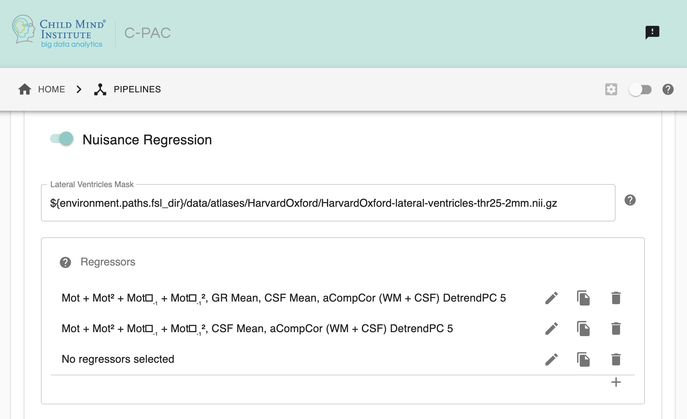
Run Nuisance Signal Correction - [Off, On, On/Off]: Covary out various sources of noise.
Lateral Ventricles Mask (Standard Space) - [path, None]: A binary mask of the lateral ventricles. If choosing None, no lateral ventricles mask will be applied.
Select Regressors: - [checkbox: compcor, wm, csf, global, pc1, motion, linear, quadratic]: Clicking on the + icon to the right of the box here will bring up a dialog where you can check off which nuisance variables you would like to include. You may generate multiple sets of nuisance regression strategies in this way. When you are done defining nuisance regression strategies, check the box next to each strategy you would like to run.
Configuring Temporal Filtering Options
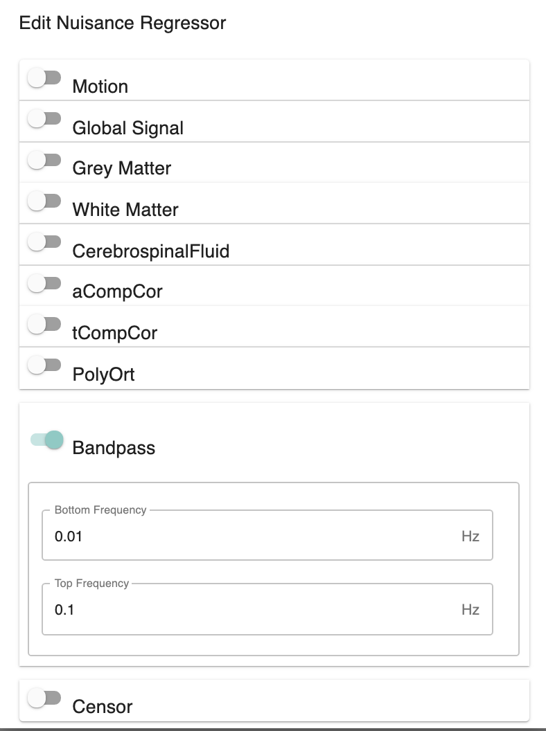
Run Temporal Filtering - [Off, On, On/Off]: Apply a temporal band-pass filter to functional data.
Select regressors: - [dialogue: Low-frequency cutoff, High-frequency cutoff]: Clicking on the + icon to the right of the box here will bring up a dialog where you can define the upper and lower cutoffs for the bandpass filter. You may generate multiple sets of bandpass filter strategies in this way. When you are done defining bandpasses, check the box next to each bandpass you would like to run.
Configuration Without the GUI
The following nested key/value pairs will be set to these defaults if not defined in your pipeline configuration YAML.
nuisance_corrections:
  2-nuisance_regression:

    # this is a fork point
    #   run: [On, Off] - this will run both and fork the pipeline
    run: [On]

    # switch to Off if nuisance regression is off and you don't want to write out the regressors
    create_regressors: On

    # Select which nuisance signal corrections to apply
    Regressors:

      -  Name: 'default'

         Motion:
           include_delayed: true
           include_squared: true
           include_delayed_squared: true

         aCompCor:
           summary:
             method: DetrendPC
             components: 5
           tissues:
             - WhiteMatter
             - CerebrospinalFluid
           extraction_resolution: 2

         CerebrospinalFluid:
           summary: Mean
           extraction_resolution: 2
           erode_mask: true

         GlobalSignal:
           summary: Mean

         PolyOrt:
          degree: 2

         Bandpass:
           bottom_frequency: 0.01
           top_frequency: 0.1
           method: default

      -  Name: 'defaultNoGSR'

         Motion:
           include_delayed: true
           include_squared: true
           include_delayed_squared: true

         aCompCor:
           summary:
             method: DetrendPC
             components: 5
           tissues:
             - WhiteMatter
             - CerebrospinalFluid
           extraction_resolution: 2

         CerebrospinalFluid:
           summary: Mean
           extraction_resolution: 2
           erode_mask: true

         PolyOrt:
          degree: 2

         Bandpass:
           bottom_frequency: 0.01
           top_frequency: 0.1
           method: default

    # Standard Lateral Ventricles Binary Mask
    # used in CSF mask refinement for CSF signal-related regressions
    lateral_ventricles_mask: $FSLDIR/data/atlases/HarvardOxford/HarvardOxford-lateral-ventricles-thr25-2mm.nii.gz

    # Whether to run frequency filtering before or after nuisance regression.
    # Options: 'After' or 'Before'
    bandpass_filtering_order: 'After'

    # Process and refine masks used to produce regressors and time series for
    # regression.
    regressor_masks:

      erode_anatomical_brain_mask:

        # Erode binarized anatomical brain mask. If choosing True, please also set seg_csf_use_erosion: True; regOption: niworkflows-ants.
        run: Off

        # Erosion proportion, if using erosion.
        # Default proportion is 0 for anatomical brain mask.
        # Recommend that do not use erosion in both proportion and millimeter method.
        brain_mask_erosion_prop : 0

        # Erode brain mask in millimeter, default of brain is 30 mm
        # brain erosion default is using millimeter erosion method when use erosion for brain.
        brain_mask_erosion_mm : 30

        # Erode binarized brain mask in millimeter
        brain_erosion_mm: 0

      erode_csf:

        # Erode binarized csf tissue mask.
        run: Off

        # Erosion proportion, if use erosion.
        # Default proportion is 0 for CSF (cerebrospinal fluid)  mask.
        # Recommend to do not use erosion in both proportion and millimeter method.
        csf_erosion_prop : 0

        # Erode brain mask in millimeter, default of csf is 30 mm
        # CSF erosion default is using millimeter erosion method when use erosion for CSF.
        csf_mask_erosion_mm: 30

        # Erode binarized CSF (cerebrospinal fluid)  mask in millimeter
        csf_erosion_mm: 0

      erode_wm:

        # Erode WM binarized tissue mask.
        run: Off

        # Erosion proportion, if use erosion.
        # Default proportion is 0.6 for White Matter mask.
        # Recommend to do not use erosion in both proportion and millimeter method.
        # White Matter erosion default is using proportion erosion method when use erosion for White Matter.
        wm_erosion_prop : 0.6

        # Erode brain mask in millimeter, default of White Matter is 0 mm
        wm_mask_erosion_mm: 0

        # Erode binarized White Matter mask in millimeter
        wm_erosion_mm: 0

      erode_gm:

        # Erode GM binarized tissue mask.
        run: Off

        # Erosion proportion, if use erosion.
        # Recommend to do not use erosion in both proportion and millimeter method.
        gm_erosion_prop : 0.6

        # Erode brain mask in millimeter, default of csf is 30 mm
        gm_mask_erosion_mm: 30

        # Erode binarized White Matter mask in millimeter
        gm_erosion_mm: 0
An example of a custom regressor with one file:
nuisance_corrections:
  2-nuisance_regression:
    Regressors:
      - Name: 'first_custom_regressor'
        Custom:
          - file: custom_signal.1D
            convolve: true
An example of nuisance regressors
The following box contains an example of a TSV file generated by C-PAC with the regressors used on nuisance regression.
# CPAC 1.4.1
# Nuisance regressors:
# RotY     RotYBack    RotYSq    RotYBackSq    RotX      RotXBack    RotXSq    RotXBackSq    RotZ      RotZBack    RotZSq    RotZBackSq    Y          YBack      YSq       YBackSq    X          XBack      XSq       XBackSq    Z          ZBack      ZSq       ZBackSq    aCompCorDetrendPC0    aCompCorDetrendPC1    aCompCorDetrendPC2    aCompCorDetrendPC3    aCompCorDetrendPC4    CerebrospinalFluidMean
-0.0276    0           0.0007    0             0.1954    0           0.0381    0             0.0488    0           0.0023    0             -0.3694    0          0.1364    0          -0.0061    0          0.0000    0          -0.3843    0          0.1476    0          -0.0458               0.0335                -0.0736               0.0579                -0.0114               10392.7714
-0.0192    -0.0276     0.0003    0.0007        0.2613    0.1954      0.0682    0.0381        0.0774    0.0488      0.0059    0.0023        -0.4328    -0.3694    0.1873    0.1364     0.0202     -0.0061    0.0004    0.0000     -0.3547    -0.3843    0.1258    0.1476     -0.1048               0.0727                -0.2194               0.1391                0.0235                10432.6865
-0.0394    -0.0192     0.0015    0.0003        0.1324    0.2613      0.0175    0.0682        0.0132    0.0774      0.0001    0.0059        -0.3399    -0.4328    0.1155    0.1873     -0.0262    0.0202     0.0006    0.0004     -0.3366    -0.3547    0.1132    0.1258     -0.1030               0.0668                -0.1124               0.0937                0.0553                10460.6806
-0.0394    -0.0394     0.0015    0.0015        0.1597    0.1324      0.0255    0.0175        0.0389    0.0132      0.0015    0.0001        -0.3419    -0.3399    0.1168    0.1155     0.0004     -0.0262    0.0000    0.0006     -0.3387    -0.3366    0.1147    0.1132     -0.0984               0.0633                -0.1343               0.1038                0.0736                10421.9697
-0.0232    -0.0394     0.0005    0.0015        0.1393    0.1597      0.0194    0.0255        0.0316    0.0389      0.0009    0.0015        -0.3486    -0.3419    0.1215    0.1168     -0.0081    0.0004     0.0000    0.0000     -0.3391    -0.3387    0.1149    0.1147     -0.0924               0.0698                -0.0869               0.1085                0.0369                10433.9453
-0.0225    -0.0232     0.0005    0.0005        0.1565    0.1393      0.0244    0.0194        0.0339    0.0316      0.0011    0.0009        -0.3828    -0.3486    0.1465    0.1215     -0.0033    -0.0081    0.0000    0.0000     -0.3498    -0.3391    0.1223    0.1149     -0.1071               0.0753                -0.0597               0.1258                -0.0705               10426.4130
-0.0233    -0.0225     0.0005    0.0005        0.1494    0.1565      0.0223    0.0244        0.0288    0.0339      0.0008    0.0011        -0.3405    -0.3828    0.1159    0.1465     -0.0062    -0.0033    0.0000    0.0000     -0.3458    -0.3498    0.1195    0.1223     -0.1158               0.0549                -0.1046               0.0821                -0.0871               10445.0371
Configuring Median Angle Correction Options
Warning
median angle correction functionality was removed in C-PAC v1.8.0.
External Resources
References
Ashby, F.G., (2011). Preprocessing. In Statistical Analysis of MRI Data. Cambridge: Cambridge University Press.
Cordes, D., Haughton, V. M., Arfanakis, K., Carew, J. D., Turski, P. A., Moritz, C. H., Quigley, M. A., et al. (2001). Frequencies contributing to functional connectivity in the cerebral cortex in “resting-state” data. AJNR. American journal of neuroradiology, 22(7), 1326–1333.
Dagli, M.S., Ingeholm, J.E., Haxby, J.V., 1999. Localization of cardiac-induced signal change in fMRI. NeuroImage 9, 407–415.
Davey, C. E., Grayden, D. B., Egan, G. F., & Johnston, L. A. (2012). Filtering induces correlation in fMRI resting state data. Neuroimage. doi:10.1016/j.neuroimage.2012.08.022 Fox, M.D., Snyder, A.Z., Vincent, J.L., Corbetta, M., Van Essen, D.C., Raichle, M.E., 2005. The human brain is intrinsically organized into dynamic, anticorrelated functional networks. Proc Natl Acad Sci U S A 102, 9673-9678.
Fox, M.D., Zhang, D., Snyder, A.Z., Raichle, M.E., 2009. The global signal and observed anticorrelated resting state brain networks. J Neurophysiol 101, 3270-3283.
Friston, K. J., Williams, S., Howard, R., Frackowiak, R. S., & Turner, R. (1996). Movement-related effects in fMRI time-series. Magnetic Resonance in Medicine, 35(3), 346–355.
Gee, D. G., Biswal, B. B., Kelly, C., Stark, D. E., Margulies, D. S., Shehzad, Z., Uddin, L. Q., et al. (2011). Low frequency fluctuations reveal integrated and segregated processing among the cerebral hemispheres. Neuroimage, 54(1), 517–527.
He Hongjian, Liu Thomas T., A geometric view of global signal confounds in resting-state functional MRI, NeuroImage, Volume 59, Issue 3, 1 February 2012, Pages 2339-2348
Murphy, K., Birn, R.M., Handwerker, D.A., Jones, T.B., Bandettini, P.A., 2009. The impact of global signal regression on resting state correlations: are anti-correlated networks introduced? Neuroimage 44, 893-905.
Power, J.D., Barnes, K.A., Snyder, A.Z., Schlaggar, B.L., Petersen, S.E., 2011. Spurious but systematic correlations in functional connectivity MRI networks arise from subject motion. Neuroimage 59, 2142-2154.
Power, J.D., Barnes, K.A., Snyder, A.Z., Schlaggar, B.L., Petersen, S.E., 2012. Steps toward optimizing motion artifact removal in functional connectivity MRI; a reply to Carp. Neuroimage.
Saad, Z.S., Gotts, S.J., Murphy, K., Chen, G., Jo, H.J., Martin, A., Cox, R.W., 2012. Trouble at rest: how correlation patterns and group differences become distorted after global signal regression. Brain Connect 2, 25-32.
Satterthwaite, T.D., Wolf, D.H., Loughead, J., Ruparel, K., Elliott, M.A., Hakonarson, H., Gur, R.C., Gur, R.E., 2012. Impact of in-scanner head motion on multiple measures of functional connectivity: Relevance for studies of neurodevelopment in youth. Neuroimage 60, 623-632.
Schroeder, C. E., & Lakatos, P. (2009). Low-frequency neuronal oscillations as instruments of sensory selection. Trends in neurosciences, 32(1), 9–18. doi:10.
Smith, AM, Lewis, BK, Ruttimann, UE, Ye, FQ, Sinnwell, TM, Yang, Y, Duyn, JH, & Frank, JA. 1999. Investigation of low frequency drift in fMRI signal. Neuroimage, 9, 526–33.
Thomas, C.G., Harshman, R.A., Menon, R.S., 2002. Noise reduction in BOLD-based fMRI using component analysis. NeuroImage 17 (3), 1521–1537.
Van Dijk, K.R., Sabuncu, M.R., Buckner, R.L., 2012. The influence of head motion on intrinsic functional connectivity MRI. Neuroimage 59, 431-438.
Wager, T.D., Hernandes, L., Jonides, J., and Lindquist, M., Elements of Functional Neuroimaging. In Cacioppo, J.T., Tassinary, L.G., and Berntson, G.G., (2007) Handbook of Psychophysiology, Third Edition.
Weissenbacher, A., Kasess, C., Gerstl, F., Lanzenberger, R., Moser, E., Windischberger, C., 2009. Correlations and anticorrelations in resting-state functional connectivity MRI: a quantitative comparison of preprocessing strategies. Neuroimage 47, 1408-1416
Windischberger, C., Langenberger, H., Sycha, T., Tschernko, E.M., Fuchsjager-Mayerl, G., Schmetterer, L., Moser, E., 2002. On the origin of respiratory artifacts in BOLD-EPI of the human brain. Magn. Reson. Imaging 20, 575–582.
Yan, C., Liu, D., He, Y., Zou, Q., Zhu, C., Zuo, X., Long, X., et al. (2009). Spontaneous brain activity in the default mode network is sensitive to different resting-state conditions with limited cognitive load. PLoS ONE, 4(5), e5743.
Zang, Y.-F., He, Y., Zhu, C.-Z., Cao, Q.-J., Sui, M.-Q., Liang, M., Tian, L.-X., et al. (2007). Altered baseline brain activity in children with ADHD revealed by resting-state functional MRI. Brain & development, 29(2), 83–91.
Zuo, X.-N., Di Martino, A., Kelly, C., Shehzad, Z. E., Gee, D. G., Klein, D. F., Castellanos, F. X., et al. (2010). The oscillating brain: complex and reliable. Neuroimage, 49(2), 1432–1445.